George Monbiot meets ... Fatih Birol on video for 12 minutes.
Accompanying story here.
Monday, December 15, 2008
Friday, December 12, 2008
 Bee petroleum company is a major branch of Bee group. Started in 1995 and is the only Sudanese oil company that’s working in the field of using LPG Liquefied Petroleum Gas to operate petrol cars. The pioneering project is having positive impact on the Sudanese economy, environment and technological advancement. Bee Aviation is part of Bee Petroleum Company.As a national petroleum company, we would like to join the leaders within the Aviation industry in Sudan. To work as a team setting standards that will not only meet local industry and international statutory regulations but enhance safety operation and protect the environment.Bee Aviation tried to start were the industry ended. We have taken all necessary measures to promote operating standards, procedures and practices in accordance with changes in company policy, changes in technology and statutory local and international regulations of joint standard operating system.
Wednesday, December 10, 2008

Ceypetco-Aviation of Ceylon Petroleum Corporation has a monopoly in Aviation fuel handling in Sri Lanka provides round the clock aviation refuelling services at Bandaranaike International Airport, Katunayake. Refueling clean & dry Aviation Fuels, on latest specifications to the right aircraft & right time economically safely & environmental friendly is the main task of ceypetco aviation. Domestic flights and some nominated foreign military aircraft are provided with refuelling services at Ratmalana airport and it is a daytime operation.Aviation Fuel cleanliness and freedom from contamination is the most important consideration for modern aircraft since it directly affects aircraft engine life & aircraft safety and influences maintenance cost. Therefore, quality control and maintenance is one of the most important aspects in aviation fuel handling. Aviation Jet fuel is produced at the Ceypetco refinery according to the latest specification checklist under “Aviation Fuel Quality Requirements for Jointly Operated Systems – AFQRJOS”. The deficit as per the predicted demand is directly imported from other countries. Current demand is one million liters daily.
Tuesday, December 9, 2008
 Zhejiang Henghe Petroleum Machine Co. Ltd.
is located beside the NanXi River , which is national view with nice and sunny with breeze fresh air . The company specially produces oil storeroom fittings and greaser fittings. Such as breathe valve double doors bottom valves and all kind of tie-ins. Since establishing in 1998, the enterprise spirit is dealing with concrete matters relating to work innovation. The principle of employing persons is advocating emphasizing knowledge mastering speciality good ability. The tenet is quality the first promoting development with scientific tech developing the market with good products. With the staff hard working developing , we have made great achievements .Our products are on sales in all over the country with high reputation ,at the same time we have gradually been cooperating and communicating with the foreigners . We have been approved for AAA Capital Enterprise Advanced Enterprise Star Enterprise Civilization Enterprise for several years, besides we have gone through ISO9001:2000. As time is developing, Henghe is developing. Expecting the future, Henghe will hearten spirit, reform, develop and create Henghe refulgence. We are looking forward to your care and sustainment.
 Saudi Light Crude Oil SLCO For SaleOur supplier is ready, willing and able to enter into a contractual agreement with the Buyer for the commodity of Saudi Light Crude Oil (SLCO) (subject to availability of allocation and fulfilment of all requests and requirements of the Seller and Saudi Aramco by the Buyer).
 Tuesday, December 2, 2008
 'Statoil ASA' is a Norwegian petroleum company established in 1972. It is the largest petroleum company in the Nordic countries and Norway's largest company, employing over 25000 people. While Statoil is listed on both the Oslo Stock Exchange and the New York Stock Exchange the Norwegian state still holds majority ownership, with 64%. The main office is located in Norway's oil capital Stavanger. The name Statoil is a truncated form of ''the State's oil''.Statoil is one of the largest net sellers of crude oil in the world, and a major supplier of natural gas to the Europe an continent, Statoil also operates around 2000 service stations in 9 countries. The company's CEO from mid-2004 onwards is Helge Lund formerly CEO of Aker Kværner.In December 2006 Statoil revealed a proposal to merge with the oil business of Norsk Hydro a Norwegian conglomerate. Under the rules of the EEA the proposal was approved by the European Union on May 3, 2007 and by the Norwegian Parliament on June 8, 2007. Statoil's shareholders will hold 67.3% of the new company2 which is likely to be known as StatoilHydro. The deal is expected to close in the third quarter of 2007. If the plan goes through, the company will be the biggest offshore oil and gas company in the world.3 The company will continue having its main headquarter located in Stavanger. The international sales and marketing division will be located in Oslo with other operations located in Stavanger.
 Sunday, November 9, 2008
Comprehensive Oil Depletion Model Life-Cycle
Setting the Stage
So I have general agreement with "Dr.Greene" in that geology determines the oil depletion arc almost completely. I would even take it a step further and also claim that probability and statistics plays an even greater role. The following comprehensive framework, that has essentially described the information content of this blog the last few years, maps out what I have tried to achieve. Don't confuse this with any kind of wacked-out psychohistory-styled prediction of the future though. Although it shares some grand aspects of a statistics-based forecasting outlook, I think I know enough when to give it a rest and not to try to predict collective human actions.

I don't consider the math behind the models that difficult to understand. The two darkened bubbles above contain the mathematical foundation for parts of the discovery process along with the oil production model. Everything fits together like a glove (IMHO and after several years of effort) and the interpretations of the model replace a longstanding set of heuristics that in the past have served to cobble together a rather poorly-formed understanding of the aggregated oil production life-cycle. The last piece in the puzzle occurred in the past few months, as I tried to decipher a model for field-size distributions.
As I spent most of my time working my way backward in the oil life-cycle timeline (right to left in the above figure), I can't provide a linear description of the comprehensive model's development. In the interim, the following bullet list of links provides reference points for entry into a mind-blowing range of pessi-optimism or opto-pessimism ... depending on your point of view.
If you enjoy the art of rhetoric more than the dialectic, beware. For many, this stuff brings on MEGO, but for a few die-hards you can get your math-porn for free.
In light of this fact, it should be no surprise that the possibility that world oil production will soon reach a peak and then inexorably decline is a subject of great interest and intense debate. As noted by Dr. Greene, the “pessimists,” a somewhat pejorative label given to those who are convinced that the oil peak is imminent and that its consequences will be dire, assert that world oil supply is chiefly determined by the geology of oil resources.The term "pessimist" has no meaning anymore. Can you still call a person who questioned the run-up of hedge funds and derivatives, not to mention the stock market for the last 10+ years, a pessimist without incurring any sense of shame? All the models in that world got built to advance one motive -- that of profit, brought about by no small part greed. No one really cared whether they made sense in some theoretical framework, and why should they, since human nature would constantly batter down the model's premises in search of escape clauses. This occurred all in the nature of one-upping the next guy ... in a zero-sum game of zero-summed optimism.
So I have general agreement with "Dr.Greene" in that geology determines the oil depletion arc almost completely. I would even take it a step further and also claim that probability and statistics plays an even greater role. The following comprehensive framework, that has essentially described the information content of this blog the last few years, maps out what I have tried to achieve. Don't confuse this with any kind of wacked-out psychohistory-styled prediction of the future though. Although it shares some grand aspects of a statistics-based forecasting outlook, I think I know enough when to give it a rest and not to try to predict collective human actions.
I don't consider the math behind the models that difficult to understand. The two darkened bubbles above contain the mathematical foundation for parts of the discovery process along with the oil production model. Everything fits together like a glove (IMHO and after several years of effort) and the interpretations of the model replace a longstanding set of heuristics that in the past have served to cobble together a rather poorly-formed understanding of the aggregated oil production life-cycle. The last piece in the puzzle occurred in the past few months, as I tried to decipher a model for field-size distributions.
As I spent most of my time working my way backward in the oil life-cycle timeline (right to left in the above figure), I can't provide a linear description of the comprehensive model's development. In the interim, the following bullet list of links provides reference points for entry into a mind-blowing range of pessi-optimism or opto-pessimism ... depending on your point of view.
If you enjoy the art of rhetoric more than the dialectic, beware. For many, this stuff brings on MEGO, but for a few die-hards you can get your math-porn for free.
Saturday, November 8, 2008
Investment in Knowledge
Nate Hagens over at TOD posted a brilliant comment in response to Exxon denial:
I don't believe in any kind of investment anymore besides an investment in knowledge. Forget investing in the stock market. Forget about investing in new ways to find oil and that "Drill, Baby, Drill" crap. Forget investing in any kind of investment, except for the one between our collective two ears.
I am beginning to believe it is an advantage to NOT work in the oil industry to understand oil. These people have been wrong, are wrong, and are about to be VERY wrong with their understanding of what peak oil means. Peak Oil has many definitions, but the most common is the all time high in world annual production of crude oil. Resources have little to do with it. (There are probably 10 million earthworms on my property -but even with a team of people and the best equipment I might only get a fraction of them). Higher prices and higher technology have little to do with Peak Oil, which has to do with cheap, reliable flow rates. There is not the slightest evidence that market theories (or activities) has helped find any more oil and gas (in the United States) since price-induced drilling increases had essentially zero impact on the production (or finding) of oil and gas.
Lets scrap the word 'peak oil' for the moment. To the economists and cornucopians at Exxon, the API, the EIA, etc. I ask these questions:
1)Do you expect oil production costs to get cheaper over time?
2) Have we past the point of cheap oil? (which is what matters - who cares if we can get an extra 20 mbpd if it takes more energy, more steel, more water and costs $500 per barrel)
3)Will the energy and other resources you use to procure oil and natural gas increase or decrease in the future?
4)Irrespective of resource or reserves, what will be the highest, reasonably low priced (say under $80 cost), FLOW rate that you can consistently provide that is not subject to geopolitical disruptions at the margin? (i.e. is there a perpetual cushion in case something goes wrong)
5)What is the error band and confidence interval you assign to your above answers? Are you willing to stake the future of industrial civilization on your answers? Even if there is a 5% chance that the resources you see translate to regular, cheap, flow rates of high quality oil, that is too big of a risk for society to take (and I think it is much higher than that).
You people are asking the wrong questions, because you've been focused on what you believe is the most important aspect of the problem - where IS the oil. That is a small part of the many more important questions, yet the group think and myopia has created an enormous blindspot. A couple months ago, if I would have told you the Federal Reserve would DOUBLE its balance sheet since the end of September, would anyone have believed me? Well, they did. Rules and facts change. Correlations that worked in the past are now uncorrelated. What was uncorrelated in the past is now completely correlated. Thats why economics isn't science. Its based on a moving target. Economists at the oil companies are trained to think in resources and price, not in energy costs and externalities. They will not see this Black Swan until it bites them in the ass.
I don't believe in any kind of investment anymore besides an investment in knowledge. Forget investing in the stock market. Forget about investing in new ways to find oil and that "Drill, Baby, Drill" crap. Forget investing in any kind of investment, except for the one between our collective two ears.
Wednesday, November 5, 2008
USA Field Size Distribution
This dated paper (circa 1986) on USA oil field size has a few interesting statistics. I don't have any of the charts, but the authors roll up a few of the numbers from the curves.

The authors state that 3% of the highest rank of fields contain 80% of the oil, which includes rank up to 440 in this chart. Or this means that 20% of the oil resides in the lowest 97% of the rank.
In the last 20 years, we probably have gained a lot of extra mileage from the low volume fields, but I can't say for certain without filling in the historical data points. If someone can get a hold of this Baker paper and post some of the charts, it would help immensely.
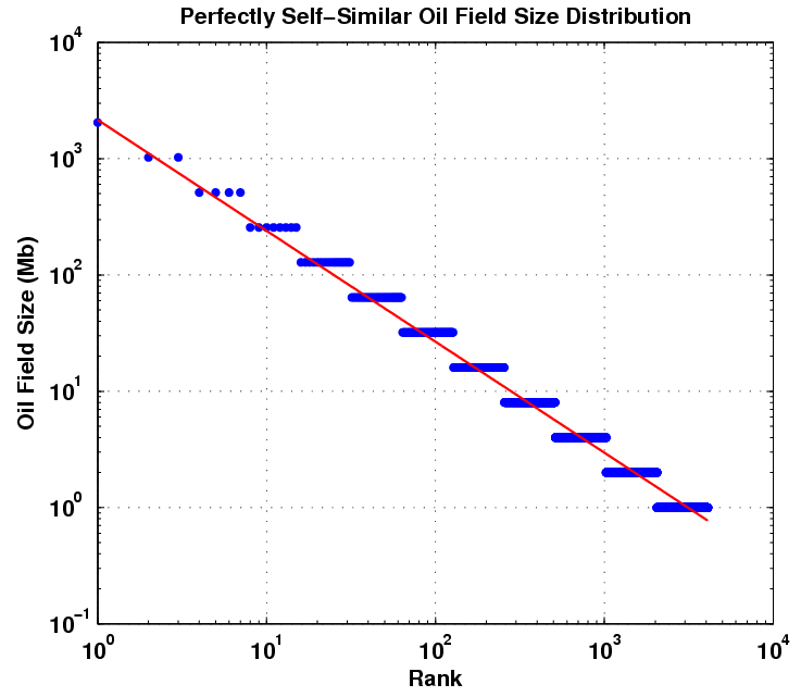
These authors also believed that the field size distribution followed a log-normal. The Dispersive Aggregation mimics the general shape of the log-normal under certain regimes, especially under a wide variance, while at the same time generating the heavy Pareto-like tail (i.e. 1/xp) that much of the data seems to indicate.

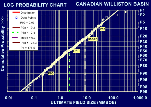
The following chart shows a cumulative field size distribution from the Canadian Williston Basin. The referenced article shows how they use a log-probability chart to map onto a log-normal curve; I pasted on a set of points corresponding to Dispersive Aggregation and as you can see, it mimics the behavior of a log-normal distribution.

The distribution of about 14,000 United States oil fields (Figure 2)--a partial sample of those in the lower 48 states--illustrates the importance of the larger fields. The sample includes almost all larger fields as known about 1970 and excludes many tiny fields as well as all of the more recent discoveries. The lower dotted line is made of 13,985 points representing the fields ordered according to increasing reserves size. Only 440 fields, or about 3%, are major ones larger than 50 million bbl. The upper curve tracks the percentage of the total oil volume occurring in fields greater than each size. From this curve, we read that the major fields, constituting only 3% of the total number, contain 80% of the total oil. Obviously, in this type of distribution one can account for the bulk of the oil by assessing the larger field possibilities only.These numbers (the 50Mb and the less than 0.1Mb) fill in the following points on the previous post.
Selecting an effective minimum field-size cutoff is very important, because it affects every major factor in the assessment--the prospects to be counted and the success and risk levels, as well as the average field size. Normally, the minimum size is taken at or just below the assumed economic minimum for the area. This approach ensures that all prospects of real interest are included. It also avoids getting bogged down in hundreds or thousands of fields that are inconsequential to early exploration stages. Furthermore, the comparative data base for assessing sub-economic fields is very weak, as the true sizes of these fields have rarely been scaled. If desired, one can assess the small fields by statistical extrapolation or by estimating a lump-sum proportion from a volume curve like that of Figure 2.
Economic limits always truncate the lower ends of observed field-size distributions (Arps and Roberts, 1958; Kaufman et al, 1975; Grender et al, 1978; Drew et al, 1982; Vinkovetsky and Rokhlin, 1982). In nature's distribution, numbers of deposits probably increase progressively in successively smaller sizes down to droplets and molecules; such a distribution is not lognormal. But we deal exclusively with artificially truncated distributions whose plots almost invariably curve upward near the low-side truncation point (upper curve, Figure 3). Our United States distribution (lower curve, Figure 2) has no data below 1,000 bbl, and many of the data points below 10,000 bbl, where the graph ends, are questionable. If the plot were continued to the left, it would ultimately curve upward at t e point of economic truncation beyond which there are no data.
We use the computational convenience of the lognormal distribution, appropriately truncated, but would not argue that this scheme is better or worse than other computational ones for strongly right-skewed distributions that have many more little fields than big fields. Some investigators (e.g., Ivanhoe, 1976; Folinsbee, 1977; Coustau, 1980) plot field size bilogarithmically against rank order. For our assessment approach, we must normalize field numbers at this stage by plotting "percent greater than" against log size. Depending on purpose and data, we may express field size as recoverable volumes of oil or of gas, or of oil plus gas on an energy-equivalent basis.
The authors state that 3% of the highest rank of fields contain 80% of the oil, which includes rank up to 440 in this chart. Or this means that 20% of the oil resides in the lowest 97% of the rank.
Up/U = (ln(1+Size/c) - 1/(1+Size/c)+ 1)/(ln(1+Max/c) - 1/(1+Max/c) + 1)I would like to make sense of this but as I don't have the original charts, I am guessing as to whether the 80% makes sense. With the Dispersive Aggregation model for the extra 21,000 fields reported, the amount of oil contributed to those above 50Mb has dropped to 50%.
| Year | Size | Fraction of Total | #Fields |
| 1986 | >50Mb | 0.80 | 13,985 |
| Today | >50Mb | 0.51 | 34,969 |
These authors also believed that the field size distribution followed a log-normal. The Dispersive Aggregation mimics the general shape of the log-normal under certain regimes, especially under a wide variance, while at the same time generating the heavy Pareto-like tail (i.e. 1/xp) that much of the data seems to indicate.
The following chart shows a cumulative field size distribution from the Canadian Williston Basin. The referenced article shows how they use a log-probability chart to map onto a log-normal curve; I pasted on a set of points corresponding to Dispersive Aggregation and as you can see, it mimics the behavior of a log-normal distribution.

Baker, R.A., H. M. Gehman, W. R. James, D. A. White, 1986,
Geologic Field Number and Size Assessment of Oil and Gas Plays,
in Oil and Gas Assessment: Methods and Applications: AAPG Studies in Geology
No. 21, p. 25 – 31.
Tuesday, November 4, 2008
Franken
Update: RECOUNT! The only reason I put up this post was that I knew it was going to be close, and Coleman is pure sleaze. I did an absentee and noticed that my ballot had ink already partially filled in the Senate column for one of the minor candidates. For once, I'd like to know if my vote got counted....
For fellow Minnesotans reading this, vote Al Franken for Senate.
Norm Coleman is a corrupt, incompetent bureaucrat who has wasted precious intellectual resources pursuing the exaggerated "Oil for Food scandal" leading up to the Iraq war. Prior to the oil crunch this summer, Oil for Food was the closest that the Republicans ever got to even talking about the global oil situation, and it turned out to be a complete smoke-screen to cover their own interests. As the previous ranking member of the Permanent Subcommittee on Investigations, we can all blame Norm Coleman for running interference on one of the most effective head-fakes perpetrated in avoiding the truth. So much for investigatin' skills there, Norm
For fellow Wright County folks, I have no doubt you will say no to the imbecilic Michele Bachmann, in favor of the El-Train.
Sunday, November 2, 2008
 Commercial Petroleum Equipment ("CPE") is a distributorship of petroleum fueling and marketing equipment, founded in 1985. Located in the Western Region of the United States, the Company maintains equipment distribution facilities in the California communities of Los Angeles and Sacramento.The Company represents in excess of three-hundred (300) manufacturers which include the finest manufacturers within the petroleum fueling industry. Categories of products include primary equipment such as dispensers, fuel control systems, hoses, nozzles and vapor recovery technologies, lights, monitoring and gauging devices, pipe, fittings, containment equipment, pumps and leak detectors, tanks, and tank hardware. CPE is well suited to provide the petroleum fueling and marketing industry products designed to meet current Federal and State regulatory guidelines within the Western Region of the United States. Currently, the primary California regulations include Assembly Bill 2481 (Continuous Secondary Monitoring), and California Air Resources Board (CARB), including Enhanced Vapor Recovery ("EVR") Phase 1 (at the tank fill), On Board Refueling Vapor Recovery Compatibility ("ORVR"), and Enhanced Vapor Recovery ("EVR") Phase II (at the dispenser), including In-Station Diagnostics ("ISD").
Wednesday, October 29, 2008
Significant, no hyperbole
Does anybody else even look at this stuff? Here we have one of the biggest issues facing the world, that of peak oil, and we don't even know how to analyze the data. Sigh. Oh well, here we go once again.
Let us look at the Dispersive Discovery model and the relationship describing cumulative reserve growth for a region:
From noting in the last post that this same dependence can occur for field sizes, I realized that an interesting mapping into reciprocal space makes these curves a lot easier to visualize and to extrapolate from. So instead of plotting t against U, we plot 1/t against 1/U

For field size distributions, it looks like this on a log-log plot. This shows up clearly as a straight line over the entire range of the reciprocal values for the variants, if you pull the constant term into one of the two variants. This works out very well for size distributions if we scale the values to an asymptotic cumulative probability of 1.

Laherrere has long referred to "hyperbolic" plots in fitting to creaming curves. If you Google for hyperbolic Laherrere, you will find several PDF files where he describes how well he can match the growth temporal behavior to one or more "hyperbolic" curves. However, I can find no mention of Laherrere's description or derivation of the hyperbolic other than its use as a heuristic. I posted about Laherrere's use of hyperbolic curves before without understanding what he meant by them. Even the thoroughly discredited cornucopian Michael Lynch could not find an explanation:

I have no doubt that Laherrere's hyperbolas map precisely into the linear Dispersive Discovery curves. I just find it unfortunate that it has taken this long to figure this key piece of the puzzle out. So we have turned the hyperbolic fit heuristic into a model which comes about from a well understood physical process, that of Dispersive Discovery.
On another positive note, I think the reciprocal fitting (Dispersion Linearization) may become just as popular as Hubbert Linearization. From what I have gathered, people seem to appreciate straight lines more than curves. Herewith, from a classic Simpson's episode:
Let us look at the Dispersive Discovery model and the relationship describing cumulative reserve growth for a region:
DD(t) = 1 / (1/L + 1/kt) => Ureserve(t)From noting in the last post that this same dependence can occur for field sizes, I realized that an interesting mapping into reciprocal space makes these curves a lot easier to visualize and to extrapolate from. So instead of plotting t against U, we plot 1/t against 1/U
1/U(t) = 1/L + 1/ktOn a linear-linear x-y plot where x maps into 1/t and y into 1/U, the linear curve looks like this:
For field size distributions, it looks like this on a log-log plot. This shows up clearly as a straight line over the entire range of the reciprocal values for the variants, if you pull the constant term into one of the two variants. This works out very well for size distributions if we scale the values to an asymptotic cumulative probability of 1.
Laherrere has long referred to "hyperbolic" plots in fitting to creaming curves. If you Google for hyperbolic Laherrere, you will find several PDF files where he describes how well he can match the growth temporal behavior to one or more "hyperbolic" curves. However, I can find no mention of Laherrere's description or derivation of the hyperbolic other than its use as a heuristic. I posted about Laherrere's use of hyperbolic curves before without understanding what he meant by them. Even the thoroughly discredited cornucopian Michael Lynch could not find an explanation:
No explanation is given for the 'hyperbolic model' or why ordering by size is more appropriate than by date of discovery.I always assumed that a hyperbolic function either meant a slice through a conic section or this type of dependence:
y = 1 / x + c1 / y = 1 / x + cThe following graph shows a typical Laherrere creaming curve analysis, where he fits to a couple of hyperbolic functions. Note that he refers to "hyperbola" in the legend. As the mellon-colored curve I plot the Dispersive Discovery cumulative . I had to slide it off Laherrere's hyperbola curve slightly since the two match exactly, which means that you couldn't tell the two apart and one curve would obscure the other.
I have no doubt that Laherrere's hyperbolas map precisely into the linear Dispersive Discovery curves. I just find it unfortunate that it has taken this long to figure this key piece of the puzzle out. So we have turned the hyperbolic fit heuristic into a model which comes about from a well understood physical process, that of Dispersive Discovery.
On another positive note, I think the reciprocal fitting (Dispersion Linearization) may become just as popular as Hubbert Linearization. From what I have gathered, people seem to appreciate straight lines more than curves. Herewith, from a classic Simpson's episode:
Professor Frink: [drawing on a blackboard] Here is an ordinary square....I am currently reading one of Professor Deirdre McCloskey's rants against non-scientific method mumbo-jumbo and feel a bit better at fighting the good fight against using arbitrary heuristics and qualitative analysis. Yet, in the long run, will anyone really care unless you can simplify it to two points on a line segment?
Police Chief Wiggum: Whoa, whoa - slow down, egghead!
Saturday, October 25, 2008

Branding and product supply of your station through a custom brand and image development, or through one of the established names in the industry, including Shell, Chevron, Texaco, and Citgo.
• Turn-key solutions to site development and/or renovation, through design and construction of state-of-the-art retail gas stations. Our designs are based on detailed location engineering and marketing analysis, traffic pattern study, demographic site survey, and construction cost control and management. We offer plans with a variety of modern facilities, including convenience stores, Dunkin’ Donuts & Baskin Robbins Franchises, QSR, service bays, and car washes.
• Business modeling, planning, and investment evaluation for all new projects developed through our dealers and business partners.
• Project financing, loan packaging, and innovative project funding.
• Facility upgrade, renovation, and automation.
• Fuel procurement, delivery, and management.
• State-of-the-art automated, remote, and real-time fuel inventory control to monitor, detect, and report inventory irregularities. These systems can also poll and log alarms, perform leak tests, and provide water level monitoring.
• Fuel cost management and control solutions through innovative methods utilizing available instruments in financial markets such as future contracts, options, and hedging.
• Station management services, including consolidated billing, reporting, and financial analysis.
• Environmental management solutions and compliance services.
• Fleet fueling services.
• Equipment sales, services, repair, and maintenance management.
• Back office integrated accounting and financial solutions that include consolidated invoicing, accounts payable, payroll, tax management, vendor relations, auditing, reporting, data storage, and credit card programs.
Friday, October 24, 2008
Estimating URR from Dispersive Field Size Aggregation
This post continues from the analysis of oil field size distribution from a few days ago. That discussion ended with questions regarding the utility of the analysis for arbitrary regions. It seemed to work well for North Sea oil but eyeballing for Mexico, the Parabolic Fractal Law looked a better empirical fit.

I did not talk much about the statistics of the rank histograms in the previous post. To remedy that I ran a few Monte Carlo simulations to determine what noise we can expect on the histograms. In particular, I went back to the North Sea data. The figure below shows a Monte Carlo run for the Dispersive Aggregation model where I sampled from the inverted distribution with P acting as a stochastic variate:

One can linearize this curve by taking the reciprocals of the variates and replotting. Note the sparseness of the endpoints which means that random fluctuations could change the local slope significantly (which has big implications for the Parabolic Fractal Model as well).
Plotting the MC data simulated for 430 point on top of the actual North Sea data and we get this:

The following figure gives a range for the single adjustable parameter in the model. For the North Sea oil, I replotted using the MaxRank and two values of C which bounded the maximum value.

The parameter

One can try to estimate URR from the closed-form solution but as I said before, the lack of a "top" to the data makes it unreliable. The actual distribution goes like 1/Size so that this integrates to the logarithm of a potentially large number -- in other words, it diverges. So unless one can put a cap on a maximum field size, ala the PFM's curvature, the URR can look infinite. From the model's perspective, one can emulate this behavior by not allowing a narrow window of probability for those large reservoir sizes.
In terms of geological time, we have one finish line, corresponding to the current time. But the growth lifetimes forr the dispersion to occur correspond roughly to all the points between now and the early history of oil formation some 300 million years ago. So we have to integrate to average out these times.
We essentially blank-out a probability window for field sizes above a certain value. This gives the following from the Dispersion relation:

Converting this graph to a rank histogram and you can notice an interesting stretching going on. Since we do have a constraint on field size, we can calculate an equivalent URR for the area under the curve.
We need to use the rank histogram to get the counting correct. Then the URR derives to:
To test the model against reality, I retrieved field size data from Khebab's post on oil field sizes and Laherrere's paper on "Estimates of Oil Reserves".

For Norway (courtesy of Khebab and Laherrere) we get the following two curves with data separated in time by several years. Note how the Maximum Rank shifts right as the value of C grows with time. Actually this shows that we may have some difficulty in separating out the decision of not developing smaller fields with an actual physical limit on the number of small fields that we count as production-level discoveries. (Caution: The values for C are in Gb, so they have to be mutiplied by 1000 to match the other C's in this post)
The World data plot (excluding USA and Canada) from Laherrere does not collect rank info from the smaller oil fields, so the vertical asymptote shown here gives a prediction of a Maximum Rank, approximately 9000 fields worldwide.

This gives a range in URR's from 1100 Gb to 1850 Gb, for values of C from 15 to 25 and a Maximum Field size of 250 Gb. I estimated the MaxRank for this model from Robelius' thesis.

Niger Delta data does not work very well at all. This could potentially work well as a candidate for constrained reservoir sizes, yet we can not rule out the possibility that some large fields have avoided discovery thus far.

I haven't found a field size distribution yet for the USA alone, but I generated the following figure as a prediction. I used a maximum rank of 34500 from Robelius's thesis and came up with two curves, with one assuming a maximum field size of 10 Gb (lower curve). The latter corresponds to a URR of 185 Gb. If I used C=0.7 and Max Field of 15 Gb, then I get URR pf 217 Gb. Ideally, I would like to get data from the USA (fat chance) to see how closely the Dispersive theory will agree with such a large (34,500) statistical sample.

Overall, most of the characteristic size (C) parameters for all the field size distribution curves fall in the range of 15 to 30 Mb (Siberia at 44), except for the USA which looks definitely less than 1 Mb. What exactly does this mean? For one, it means that the USA has a much higher fraction of smaller oil fields than the rest of the world. Is this actually due to more resources invested into prospecting for smaller oil fields than the rest of the world? Or is it because the USA has a physical preponderance of smaller oil fields? I don't know. Yet, the latter does make some sense considering how much more reserve growth that the USA shows than the rest of the world (and the number of stripper wells we have). Slower reserve growth occurs for exactly the same reason -- slower relative dispersion in comparison to distance involved -- that it does for dispersive aggregation. After all, I constructed the underlying model in identical ways, substituting natural discovery in Dispersive Aggregation for man-made discovery in Dispersive Reserve Growth.
You can well ask why the curve nosedives so steeply near the maximum rank. It really only looks that way on a log-log plot. Actually the distribution flattens out near zero and this creates a graphical illusion of sorts. The dispersion model says that up to a certain recent time in geological history, many of the oil fields have not started dispersing significantly -- at this point the slow rates have not yet made their impact and the fast rates haven't had any time to evolve. This manifests as an unknown distribution of sizes for oil fields before this point. (If you plot a population's yearly income on a rank histogram you will see this same effect, in this case due to a similar truncation due to a slow income growth early in a career). The USA field essentially has a much slower dispersive evolution than the rest of the world, so we have a much higher fraction of small fields that have not aggregated.
The Dispersive Field Size Aggregation falls into the Dispersion Theory category of models that seem to have a high degree of cohesion and connectedness. It looks like we can actually connect the dots from dispersive field sizes to the Logistic shape of the Hubbert Peak since the underlying statistical fundamentals have much commonality in terms of temporal and spatial behaviors. For now I can't find a derivation of the Parabolic Fractal Law, which to me looks like a heuristic. I always base my observations on a model. I don't lock-step believe in heuristics, mainly because I have a perhaps unhealthy obsession with understanding why a heuristic works at all (review my railing against the "derivation" of the Logistic that I have frequently written about, until I figured it out to my satisfaction). By definition, a heuristic does not have to explain anything, it just has to describe the results. And describing the results in a mathematical equation does not cut it for me. For all I know, all the Wall Street quantitative analysts (the "quants") have based all their derivative and hedge fund "models" on heuristics -- and look a where that has got us.
In my mind, Dispersive Aggregation makes a lot of sense and it seems to fit the data. I smell another TOD post brewing.
I did not talk much about the statistics of the rank histograms in the previous post. To remedy that I ran a few Monte Carlo simulations to determine what noise we can expect on the histograms. In particular, I went back to the North Sea data. The figure below shows a Monte Carlo run for the Dispersive Aggregation model where I sampled from the inverted distribution with P acting as a stochastic variate:
Size=c*(1/P-1) where P=[0..1]One can linearize this curve by taking the reciprocals of the variates and replotting. Note the sparseness of the endpoints which means that random fluctuations could change the local slope significantly (which has big implications for the Parabolic Fractal Model as well).
Plotting the MC data simulated for 430 point on top of the actual North Sea data and we get this:
The following figure gives a range for the single adjustable parameter in the model. For the North Sea oil, I replotted using the MaxRank and two values of C which bounded the maximum value.
The parameter
C acts like a multiplier so it essentially moves the curves up or down on a log-log plot.One can try to estimate URR from the closed-form solution but as I said before, the lack of a "top" to the data makes it unreliable. The actual distribution goes like 1/Size so that this integrates to the logarithm of a potentially large number -- in other words, it diverges. So unless one can put a cap on a maximum field size, ala the PFM's curvature, the URR can look infinite. From the model's perspective, one can emulate this behavior by not allowing a narrow window of probability for those large reservoir sizes.
In terms of geological time, we have one finish line, corresponding to the current time. But the growth lifetimes forr the dispersion to occur correspond roughly to all the points between now and the early history of oil formation some 300 million years ago. So we have to integrate to average out these times.
Cumulative (PDF(Size)) =where the value of Now you can consider as roughly 300 million years from the start of the oil age. Small values of T correspond to the start of dispersion at longer times ago and higher values result in values closer to the present (Now) time. The number T itself scales proportionately to the rank index on a field distribution plot if dispersion proceeds more or less linearly with time (kT ~ Size). Also, a rank value of 1 corresponds to the largest value on a rank histogram plot from which can estimate Maximum Field Size. Given a mature enough set of field data, this provides close to the ceiling for where fields cannot aggregate.
Integral (PDF(Size)dSize) from 0 .. Now =
Integral (PDF(kt)dt) from 0 .. Now
We essentially blank-out a probability window for field sizes above a certain value. This gives the following from the Dispersion relation:
The following set of curves shows the dispersive aggregate growth models under the conditions of a maximum field size constraint, set to L=1000.P(Size) = K*Integral (C/(Size+C)^2 dSize) from Size = [0..L]
P(Size) = Size*(L+C)/(Size+C)/L
... invertingwhere P=[0..1]
Size = C*P/(1+C/L-P)
Converting this graph to a rank histogram and you can notice an interesting stretching going on. Since we do have a constraint on field size, we can calculate an equivalent URR for the area under the curve.
We need to use the rank histogram to get the counting correct. Then the URR derives to:
URR = MaxRank * C * ((1+C/L)*ln (1+L/C) - 1)for most cases, this approximates to:
URR ~ MaxRank * C * (ln (L/C) - 1)Note that the URR has a stronger dependence on the parameter C than the maximum field size L , which has a weak logarithmic behavior. I will discuss the case of the USA further down this post but keep in mind that Americans have more oil fields by far than anyone else in the world, i.e. a huge MaxRank, yet our URR does not swamp out everyone else.
To test the model against reality, I retrieved field size data from Khebab's post on oil field sizes and Laherrere's paper on "Estimates of Oil Reserves".
- North Sea (see above)
- Mexico
- Norway
- World (minus USA/Canada)
- West Siberia
- Niger
- USA

For Norway (courtesy of Khebab and Laherrere) we get the following two curves with data separated in time by several years. Note how the Maximum Rank shifts right as the value of C grows with time. Actually this shows that we may have some difficulty in separating out the decision of not developing smaller fields with an actual physical limit on the number of small fields that we count as production-level discoveries. (Caution: The values for C are in Gb, so they have to be mutiplied by 1000 to match the other C's in this post)
 Old data |  Recent data |
The World data plot (excluding USA and Canada) from Laherrere does not collect rank info from the smaller oil fields, so the vertical asymptote shown here gives a prediction of a Maximum Rank, approximately 9000 fields worldwide.
This gives a range in URR's from 1100 Gb to 1850 Gb, for values of C from 15 to 25 and a Maximum Field size of 250 Gb. I estimated the MaxRank for this model from Robelius' thesis.
An article by Ivanhoe and Leckie (1993) in Oil & Gas Journal reported the total amount of oil fields in the world to almost 42000, of which 31385 are in the USA. According to the latest Oil & Gas Journal worldwide production survey, the total number of oil fields in the USA is 34969 (Radler, 2006). The number of fields outside the USA is estimated to 12500, which is in good accordance with the number 12465 given by IHS Energy (Chew, 2005). Thus, the total number of oil fields in the world is estimated to 47 500.From Khebab, the PFM gives a low end estimate ignoring the missing parts of the rank histogram:
Using his (Laherrere's) parameters, we can compute a world URR (excluding the US and Canada, conventional oil) equals to 1.250 Trillions of Barrels (Tb) without considering oil fields with sizes below 50 Mb.This chart from West Siberia bins histogram data on a linear plot.
Niger Delta data does not work very well at all. This could potentially work well as a candidate for constrained reservoir sizes, yet we can not rule out the possibility that some large fields have avoided discovery thus far.

I haven't found a field size distribution yet for the USA alone, but I generated the following figure as a prediction. I used a maximum rank of 34500 from Robelius's thesis and came up with two curves, with one assuming a maximum field size of 10 Gb (lower curve). The latter corresponds to a URR of 185 Gb. If I used C=0.7 and Max Field of 15 Gb, then I get URR pf 217 Gb. Ideally, I would like to get data from the USA (fat chance) to see how closely the Dispersive theory will agree with such a large (34,500) statistical sample.
Overall, most of the characteristic size (C) parameters for all the field size distribution curves fall in the range of 15 to 30 Mb (Siberia at 44), except for the USA which looks definitely less than 1 Mb. What exactly does this mean? For one, it means that the USA has a much higher fraction of smaller oil fields than the rest of the world. Is this actually due to more resources invested into prospecting for smaller oil fields than the rest of the world? Or is it because the USA has a physical preponderance of smaller oil fields? I don't know. Yet, the latter does make some sense considering how much more reserve growth that the USA shows than the rest of the world (and the number of stripper wells we have). Slower reserve growth occurs for exactly the same reason -- slower relative dispersion in comparison to distance involved -- that it does for dispersive aggregation. After all, I constructed the underlying model in identical ways, substituting natural discovery in Dispersive Aggregation for man-made discovery in Dispersive Reserve Growth.
You can well ask why the curve nosedives so steeply near the maximum rank. It really only looks that way on a log-log plot. Actually the distribution flattens out near zero and this creates a graphical illusion of sorts. The dispersion model says that up to a certain recent time in geological history, many of the oil fields have not started dispersing significantly -- at this point the slow rates have not yet made their impact and the fast rates haven't had any time to evolve. This manifests as an unknown distribution of sizes for oil fields before this point. (If you plot a population's yearly income on a rank histogram you will see this same effect, in this case due to a similar truncation due to a slow income growth early in a career). The USA field essentially has a much slower dispersive evolution than the rest of the world, so we have a much higher fraction of small fields that have not aggregated.
The Dispersive Field Size Aggregation falls into the Dispersion Theory category of models that seem to have a high degree of cohesion and connectedness. It looks like we can actually connect the dots from dispersive field sizes to the Logistic shape of the Hubbert Peak since the underlying statistical fundamentals have much commonality in terms of temporal and spatial behaviors. For now I can't find a derivation of the Parabolic Fractal Law, which to me looks like a heuristic. I always base my observations on a model. I don't lock-step believe in heuristics, mainly because I have a perhaps unhealthy obsession with understanding why a heuristic works at all (review my railing against the "derivation" of the Logistic that I have frequently written about, until I figured it out to my satisfaction). By definition, a heuristic does not have to explain anything, it just has to describe the results. And describing the results in a mathematical equation does not cut it for me. For all I know, all the Wall Street quantitative analysts (the "quants") have based all their derivative and hedge fund "models" on heuristics -- and look a where that has got us.
In my mind, Dispersive Aggregation makes a lot of sense and it seems to fit the data. I smell another TOD post brewing.
Tuesday, October 21, 2008
Dispersive Discovery / Field Size convergence
 After having studied material nucleation and growth processes for a good portion of my grad school tenure, I think I can grasp some of the fundamentals that go into oil reservoir size distributions. I see many similarities between the two processes. For example, instead of individual atoms and molecules, we deal with quantities on the order of million-barrels-of-oil, yet the fundamental processes remain the same: diffusion, drift, conservation of matter, rate equations, etc. Deep physical processes go into the distribution of field sizes, yet I contend that some basic statistical ideas surrounding kinetic growth laws may prove more useful than understanding the fundamental physics of the process. To make the case even stronger, I use the same ideas from the model of Dispersive Discovery to show how the current distribution can arise; as humans sweep through a volume searching for oil, so too can oil diffuse or migrate to "discover" pockets that lead to larger reservoirs. The premise that varying rates of advance can disperse the ultimate observable measure leads to the distribution we see. For oil discovery, the amount gets dispersed with time, while with field sizes, the dispersion occurs with time as well, but we see the current density as a snapshot in a much slower glacially-paced geological time. For the latter, we will never see any changes in our lifetime, but much like tree rings and glacial cores can tell us about past Earth climates, the statistics of the size distribution can tell us about the past field size growth dynamics.
B. Michel provided a decent set of data for reservoir size distribution ranking of North Sea fields in his paper that I referenced here. Michel tried to make the point that the shape follows a Pareto distribution, which shows an inverse power law with size.

This kind of rank plot is easy to generate and shows the qualitative inverse power law, close to 1/Size in this case. The curve also displays some anomalies, primarily at the small field sizes portion and a bit at the large field sizes.
Khebab has some good background on the Pareto as well as the Parabolic Fractal Law described here. He also analyzed the log-normal used by USGS here. And he has some devised some case studies for Norway and Saudi Arabia.
 Neither the Pareto nor the Parabolic Fractal Law fit the extreme change of slope near the small field size region of the curve. The log-normal does better than this but does not universally get used (it also looks very well suited to small particle and aersol size distributions). The model I use seems to work better and it derives in a similar manner to the discovery process itself. If oil can tend to seek out itself or cluster via settling in low energy states and by increasing entropy via diffusing from regions of high concentration, this itself we can consider as a discovery process. So as an analogy I assume that oil can essentially "find" itself and thus pool up to some degree. By the same token, the ancient biological matter had a tendency to accumulate in a similar way. In any case, this process has taken place over the span of millions of years. After this "discovery" or aggregation takes place, the oil doesn't get extracted like it would in a human-accelerated discovery process but it gets stored in situ, ready to be rediscovered by humans. And of course consumed in a much shorter time than it took to generate!
The following figure takes Michel's rank histogram and exchanges the axis to convert it into a regular (binned) histogram. The fitted curve assumes Dispersive Discovery via the Laplace transform of an exponentially distributed set of points. This differs from the reserve growth of discovery only in the sense that the cumulative starts from 100% instead of zero; in other words, in a region near the origin, just about all reservoirs reach at least this size. The curve essentially describes the line 1/(1+Size/20 Mb), where 20 Mb is the characteristic dispersion size derived from the original exponential distribution used. In the case of DD, 20 Mb becomes an average equivalent size that a columnar reserve growth discovery process would need to sweep through before significant discoveries would occur. For field sizes, we can use the same argument and equate this to a natural growth accumulation, where the average growth rate would start to see the effects of aggregation above the mean.

 damped exponential distribution |  clustered distribution after accumulation |
I can see another straight line through points which would give a slope of 1/Size0.96, but in general, for this region a single parameter controls the curvature via 1/(1+Size/20 Mb). If put into the context of a time-averaged rate, where the inflection point Size = k*Time = 20 Mb, where k is in terms of average amount migrated per geological time in a region, you can get a sense of how slow this migration is. If Time is set to 300 Million years, the constant k comes out to less than 1/10 barrel per year on average. The dispersion theory gives a range as a standard deviation of this same value, which means that the rates slow to an even more apparent crawl as well as speed up enough to contribute to the super-giant fields over the course of time.
Even though the approach relies on kinetic (not equilibrium) arguments, this works out as much by a conservation of mass argument as anything else. If a volume gets completely swept out, via diffusion and seepage, and all the oil in a region congregates, it becomes the biggest possible reservoir with a rank equal to 1. Yet, it has to equal the volume of the original distribution. The curve essentially shows cross-sections of the advancing mean at various stages of time, i.e. a moving finish line. So we assume that the last, rank=1, point is the finish line. Since the dispersion assumes a constant standard deviation relative to the mean, the stationary assumption implies that the rest of the distribution fractionally scales to match the extent of the fastest flow. So I have a feeling that this recasts the fractal argument, but only adding a starting exponential distribution which eliminates the pure 1/Size dependence of the fractal or Pareto distribution.

In a global context and given enough time, this simple kinetic flow model would eventually grow to such an extent that a single large reservoir would engulf the entire world's reserves. This does not happen however and since we deal with finite time, the curve drops off at the extreme of large reservoir sizes. We can't wait for an infinite amount of time so we have never and likely will never see the biggest reservoir sizes, Black Swan events notwithstanding. So if we extended the following figure to show 1/Size dependence over an infinite range, this would of course only hold true in an infinite universe. I can't tell because of the poor statistics we have to deal with, i.e. N=small, but the supergiants might just sit at the edge of the finite time we have to deal with.
What actually happens underground? Oil does move around through the processes of drift, diffusion, gravity drainage, bouyancy, and it does this at various rates. The reason that small particles, grains, and crystals show this same type of growth also has to do with a dispersion in growth rates. Initially, all bits of material start with a nucleating site, but due to varying environmental conditions, the speed of growth starts to disperse and we end up with a range of particle sizes after a given period of time. The size distribution of many small particles and few large ones will only occur if slow growers exponentially outnumber fast growers. The same thing must happen with oil reservoirs; only a few show a path that allows exteremely "fast" accumulation ( I say "fast" because this still occurs over millions of years). From the post on marathon results dispersion, it basically demonstrates the same intuitive behavior. Only the fastest of the dispersers will maximize the amount of ground covered (or material accumulated) in a certain period of time.

The reason I wouldn't use field size distribution arguments alone to estimate URR is because no "top" exists for the cumulative size, since we do not consider the size of the container that all the fields fit in to. The Dispersive Discovery model explicitly includes a URR-style limiting container, which makes it much more useful for extrapolating future reserves. I find it interesting though in how the two approaches complement each other. Dispersive Discovery only considers the size of the container, while Dispersive Growth figures out the distribution of sizes within the container. And as long as discoveries occur in a largely unordered fashion (I assert that large oil reserves are not necessarily always found first), using the Dispersive Discovery curve makes the analysis more straightforward (no matter what the USGS says).
Khebab and Laherrere make some good points concerning the Parabolic Fractal Law as some curves show significant "bending" as this size distribution from Mexico demonstrates:
So far the Dispersive Growth field size model uses a single parameter; I figure that I have another one to spare to explain Mexico.
Sunday, October 19, 2008
Why We Can't Pump Faster
According to the Oil Shock model, to first order the rate of depletion occurs proportionately to the amount of reserve available. Overall, this number has remained high and fairly constant (I consider 5% per year high for any non-renewable resource). It takes effort to extract it substantially faster than this, but because of oil's value -- they don't call it black gold for nothing -- we never have had a reason not to extract, and so it has maintained its rate at a steady level, OPEC notwithstanding. And because the extraction rate has never varied by orders of magnitude, we have little insight into what we have in store for the future. In other words, can we actually pump faster?
The following proportionality equation forms the lowest-level building block of the Shock model.
 The characteristic solution of the first-order equation to delta function initial conditions derives to a damped exponential.
As Khebab has pointed out via the Hybrid Shock Model (HSM), this gives the behavior that production always decreases, unless additional reserves get added (the extrapolation of future reserves is the key to HSM). And if we reside near the backside of a peak and without any newly-discovered additive reserves, it will go only one way ... down.
Yet we know that plateauing of the peak will likely occur, at least at the start of any detectable decline. This will invariably come about from an increase in extraction from reserves. According to the shock model, this only increases if k increases. We can model this straightforwardly:
Notice how this gives a momentary plateau that soon gets subsumed by the relentless extractive force.
Instead of a 2nd order increase, we can try adding an exponential increase in extraction rate:
The solution to this results in a variation of the Gompertz equation:
The uptick of the plateau has now become more pronounced. Overgeneralizing, "we" can now "dial-in" the extension of the plateau "supply" by "adjusting" the extraction rate at an accelerating rate. I place air quotes around these terms because I have a feeling that (1) know one knows the feasibility of improved extractive technology and (2) it will eventually hit a hard downslope. Under the best circumstances we may prolong the plateau somewhat.
 Conversely, assuming the conditions of a non-rate limited supply, oil producers can increase their output at the whim of political decisions. No one really understands the extent of this strategy; the producers who consider oil as a cash cow will not intentionally limit production, while those who emulate OPEC cartel practices will carefully meter output to meet some geopolitical aims. In this case, shareholders demanding the maximization of profit do not play a role.
So, what is the downside of increasing the extraction rate?
Answer: The downside is the downslope. Quite literally, upping the extraction rate under a limited supply makes the downslope that much more pronounced. The Gompertz shows a marked asymmetry that more closely aligns to exponential rise and collapse than the typical symmetric Hubbert curve.
A while back I discussed the possibility of reaching TOP (see The Overshoot Point) whereby we keep trying to increase the extraction rate until the reserve completely dries up and the entire production collapses. The following curves give some pre-dated hypothetical curves for TOP. The graph on the right shows the extractive acceleration necessary to maintain a plateau. At some point the extraction rate needs to reach ridiculous levels to maintain a plateau, and if we continue with only a linear rate of increase it starts to give and the decline sets in. Clearly, this approach won't sustain itself. And if we stop the increase completely, the production falls precipitously (see the Exponential Growth + Limit curve above).
In summary, this part of the post essentially covers the same territory as my initial TOP discussion from a few years ago, but I tried to give it some mathematical formality that I essentially overlooked for quite a while.
Do we ever see the Gompertz curve in practice? I venture to guess that yes we have. Not a pleasant topic, but we should remind ourselves that fast developing extinction events may show Gompertz behavior. Oil depletion dynamics would play out similarly to sudden extinction dynamics, if and only if we assume that oil production immediately succeeded discovery and the extraction rate then started to accelerate. Then when we look at an event like passenger pigeon population (where very limited dispersion occurs), the culling production increases rapidly and then collapses as the population can't reproduce or adapt fast enough.
As a key to modeling this behavior, we strip out dispersion of discovery completely, and then provide a discovery stimulus as a delta function. For passenger pigeons the discovery occurred as a singular event along the Eastern USA during colonial times. The culling accelerated until the population essentially became extinct in the late 1800's.
To verify this in a more current context, I decided to look at the vitally important worldwide phosphate production curve. Bart Anderson at the Energy Bulletin first wrote about this last year and he provided some valuable plots courtesy of his co-author Patrick Déry. At that time, I thought we could likely do some type of modeling since the production numbers seemed so transparently available. Gail at TOD provided an updated report courtesy of James Ward which rekindled my interest in the topic. Witness that the search for phosphate started within a few decades of the discovery of oil in the middle 1800's. Therefore one may think the shape of the phosphate discovery curve might also follow a logistic like curve. But I contend that this does not occur because of accelerating extraction rates of phosphate leading to more Gompertz-like dynamics.
The first plot that provides quite a wow factor comes from phosphate production on the island of Nauru by way of Anderson and Déry.

Note that the heavy dark green line that I added to the set of curves follows a Gompertz function with an initial stimulus at around the year 1900, and an exponential increase after that point. The total reserve available defines the peak and subsequent decline. The long uptake and rapid decrease both show up much better with Gompertz growth than with the HL/Logistic growth. This does not invalidate the HL (of which Dispersive Discovery model plays a key role), but it does show where it may not work as well.
Remember that all the phosphate on that island essentially became "discovered" as a singular event in 1900 (not hard to imagine for the smallest independent republic in the world). Since that time, worldwide fertilizer production/consumption has increased exponentially reaching values of 10% growth per year before leveling off to 5% or less per year. Google
"rate of fertilizer consumption" to find more evidence.
Then if you consider that most easily accessible phosphate discoveries occurred long ago, the role of Gompertz type growth becomes more believable1. No producer had ever really over-extracted the phosphate reserves in the early years, as we would have had no place to store it, yet the growth continued as the demand for phosphate for fertilizer increased exponentially. So as the demand picked up, phosphate companies simply depleted from the reserves until they hit the diminishing return part of the curve. The producers can essentially pull phosphates out of the reserves as fast as they wanted, while oil producers became the equivalent of drinking a milkshake from a straw, as sucking harder does not help much.
For worldwide production of phosphates, applying the Gompertz growth from non-dispersive discoveries gives a more pessimistic outlook than what James Ward calculated. The following figure compares Ward's Hubbert Linearization against an eyeballed Gompertz fit. Note that both show a similar front part of the curve but the Gompertz declines much more rapidly on the backside. The wild production swings may come about from the effects of a constrained supply, something quite familiar to those following the stock market recently and the effects of constrained credit on speculative outlook.

So we have the good news and the bad news. First, the good news: oil production does not follow the Gompertz curve as of yet and we may not ever reach that potential given the relative difficulty of extracting oil at high rates. The fact that we have such a high dispersion in oil discoveries also means that the decline becomes mitigated by new discoveries. As for the bad news: easily extractable phosphate may have hit TOP. And we have no new conventional sources. And phosphate essentially feeds the world.
Read the rest of Ward's post for some hope:

1 For a quick-and-dirty way to gauge discovery events, I used Google to generate a histogram. I describe this technique here and here. For phosphates, the histogram looks like this:

Note the big spike in discoveries prior to 1900; recent large discoveries remain rare. Prospectors have long ago sniffed out most new discoveries.
Update:
Sulfur Gompertz, used in fertilizer production as well:

from http://pubs.usgs.gov/of/2002/of02-298/of02-298.pdf, ref courtesy of TOD.
The following proportionality equation forms the lowest-level building block of the Shock model.
dU/dt = -k U(t)Any shocks come about by perturbing the value of k in the equation. Painfully stating the obvious, the values of k can go up or down. Up to now the perturbations have usually spiked downward, usually from OPEC decisions. In particular, during the oil crises of the 1970's, the model showed definite glitches downward corresponding to temporary reductions in the extraction rate imposed to member countries by the cartel (of which formed the original motivation and basis of the shock model).
The characteristic solution of the first-order equation to delta function initial conditions derives to a damped exponential. U(t) = U0 e-ktwith extractive production following as the derivative of U(t) (the negative sign indicates extraction):
P(t) = -dU(t)/dt = k * U0 e-kt = k*U(t)This gets back to the original premise: "rate of depletion occurs proportionately to the amount of reserve available".
As Khebab has pointed out via the Hybrid Shock Model (HSM), this gives the behavior that production always decreases, unless additional reserves get added (the extrapolation of future reserves is the key to HSM). And if we reside near the backside of a peak and without any newly-discovered additive reserves, it will go only one way ... down.
Yet we know that plateauing of the peak will likely occur, at least at the start of any detectable decline. This will invariably come about from an increase in extraction from reserves. According to the shock model, this only increases if k increases. We can model this straightforwardly:
dU/dt = -(k + ct) U(t)Regrouping terms to integrate:
dU/U = -(k + ct)dtthis results in
ln(U) - ln(U0) = -(kt + ct2/2)
U = U0 e-(kt + ct2/2)
P(t) = (k + ct)* U0 e-(kt + ct2/2)
Notice how this gives a momentary plateau that soon gets subsumed by the relentless extractive force.
Instead of a 2nd order increase, we can try adding an exponential increase in extraction rate:
dU/U = -(k + a*ebt)dt
ln(U) - ln(U0) = -(kt + a*ebt/b)
The solution to this results in a variation of the Gompertz equation:
U = U0 e-(kt + a*ebt/b)
P(t) = (k+ a*ebt)U0 e-(kt + a*ebt/b)
The uptick of the plateau has now become more pronounced. Overgeneralizing, "we" can now "dial-in" the extension of the plateau "supply" by "adjusting" the extraction rate at an accelerating rate. I place air quotes around these terms because I have a feeling that (1) know one knows the feasibility of improved extractive technology and (2) it will eventually hit a hard downslope. Under the best circumstances we may prolong the plateau somewhat.
Conversely, assuming the conditions of a non-rate limited supply, oil producers can increase their output at the whim of political decisions. No one really understands the extent of this strategy; the producers who consider oil as a cash cow will not intentionally limit production, while those who emulate OPEC cartel practices will carefully meter output to meet some geopolitical aims. In this case, shareholders demanding the maximization of profit do not play a role.So, what is the downside of increasing the extraction rate?
Answer: The downside is the downslope. Quite literally, upping the extraction rate under a limited supply makes the downslope that much more pronounced. The Gompertz shows a marked asymmetry that more closely aligns to exponential rise and collapse than the typical symmetric Hubbert curve.
A while back I discussed the possibility of reaching TOP (see The Overshoot Point) whereby we keep trying to increase the extraction rate until the reserve completely dries up and the entire production collapses. The following curves give some pre-dated hypothetical curves for TOP. The graph on the right shows the extractive acceleration necessary to maintain a plateau. At some point the extraction rate needs to reach ridiculous levels to maintain a plateau, and if we continue with only a linear rate of increase it starts to give and the decline sets in. Clearly, this approach won't sustain itself. And if we stop the increase completely, the production falls precipitously (see the Exponential Growth + Limit curve above).
 |  |
In summary, this part of the post essentially covers the same territory as my initial TOP discussion from a few years ago, but I tried to give it some mathematical formality that I essentially overlooked for quite a while.
Do we ever see the Gompertz curve in practice? I venture to guess that yes we have. Not a pleasant topic, but we should remind ourselves that fast developing extinction events may show Gompertz behavior. Oil depletion dynamics would play out similarly to sudden extinction dynamics, if and only if we assume that oil production immediately succeeded discovery and the extraction rate then started to accelerate. Then when we look at an event like passenger pigeon population (where very limited dispersion occurs), the culling production increases rapidly and then collapses as the population can't reproduce or adapt fast enough.
As a key to modeling this behavior, we strip out dispersion of discovery completely, and then provide a discovery stimulus as a delta function. For passenger pigeons the discovery occurred as a singular event along the Eastern USA during colonial times. The culling accelerated until the population essentially became extinct in the late 1800's.
To verify this in a more current context, I decided to look at the vitally important worldwide phosphate production curve. Bart Anderson at the Energy Bulletin first wrote about this last year and he provided some valuable plots courtesy of his co-author Patrick Déry. At that time, I thought we could likely do some type of modeling since the production numbers seemed so transparently available. Gail at TOD provided an updated report courtesy of James Ward which rekindled my interest in the topic. Witness that the search for phosphate started within a few decades of the discovery of oil in the middle 1800's. Therefore one may think the shape of the phosphate discovery curve might also follow a logistic like curve. But I contend that this does not occur because of accelerating extraction rates of phosphate leading to more Gompertz-like dynamics.
The first plot that provides quite a wow factor comes from phosphate production on the island of Nauru by way of Anderson and Déry.
Note that the heavy dark green line that I added to the set of curves follows a Gompertz function with an initial stimulus at around the year 1900, and an exponential increase after that point. The total reserve available defines the peak and subsequent decline. The long uptake and rapid decrease both show up much better with Gompertz growth than with the HL/Logistic growth. This does not invalidate the HL (of which Dispersive Discovery model plays a key role), but it does show where it may not work as well.
Remember that all the phosphate on that island essentially became "discovered" as a singular event in 1900 (not hard to imagine for the smallest independent republic in the world). Since that time, worldwide fertilizer production/consumption has increased exponentially reaching values of 10% growth per year before leveling off to 5% or less per year. Google
"rate of fertilizer consumption" to find more evidence.
As a result, fertilizer trade increased from about 2 million tons in 1950 to about 40 million tons in 1986.Over this period, this rate compounds to 9% annually, clearly an exponential increase which menas that the phosphate component of fertilizer increased as well.
Then if you consider that most easily accessible phosphate discoveries occurred long ago, the role of Gompertz type growth becomes more believable1. No producer had ever really over-extracted the phosphate reserves in the early years, as we would have had no place to store it, yet the growth continued as the demand for phosphate for fertilizer increased exponentially. So as the demand picked up, phosphate companies simply depleted from the reserves until they hit the diminishing return part of the curve. The producers can essentially pull phosphates out of the reserves as fast as they wanted, while oil producers became the equivalent of drinking a milkshake from a straw, as sucking harder does not help much.
For worldwide production of phosphates, applying the Gompertz growth from non-dispersive discoveries gives a more pessimistic outlook than what James Ward calculated. The following figure compares Ward's Hubbert Linearization against an eyeballed Gompertz fit. Note that both show a similar front part of the curve but the Gompertz declines much more rapidly on the backside. The wild production swings may come about from the effects of a constrained supply, something quite familiar to those following the stock market recently and the effects of constrained credit on speculative outlook.
So we have the good news and the bad news. First, the good news: oil production does not follow the Gompertz curve as of yet and we may not ever reach that potential given the relative difficulty of extracting oil at high rates. The fact that we have such a high dispersion in oil discoveries also means that the decline becomes mitigated by new discoveries. As for the bad news: easily extractable phosphate may have hit TOP. And we have no new conventional sources. And phosphate essentially feeds the world.
Read the rest of Ward's post for some hope:
Perhaps the best way to frame the debate from here is to suggest that, like oil, the world has been endowed with a given quantity of “easy” phosphorus (e.g. rich island guano deposits in places like Nauru) that can be – and have been – mined quite rapidly, as well as a larger endowment of lower-grade phosphate rock. While the easy phosphate has passed its peak, the low-grade phosphate should be considered separately. Figure 3 shows an example forecast where the total area under both curves (equal to RURR) is 24.3 billion tonnes, but the “easy” phosphorus (purple) is 9 billion tonnes as in Figure 2. Assuming the production history is mostly related to easy phosphorus, the fitting parameters (a and k) for the “hard” phosphorus cannot be established. Therefore, the height and timing of the secondary peak are unpredictable.
1 For a quick-and-dirty way to gauge discovery events, I used Google to generate a histogram. I describe this technique here and here. For phosphates, the histogram looks like this:
Note the big spike in discoveries prior to 1900; recent large discoveries remain rare. Prospectors have long ago sniffed out most new discoveries.
Update:
Sulfur Gompertz, used in fertilizer production as well:

from http://pubs.usgs.gov/of/2002/of02-298/of02-298.pdf, ref courtesy of TOD.
Subscribe to:
Posts (Atom)