Saturday, May 29, 2010

The Word on Dispersion

Credit the Gulf oil disaster with allowing the words dispersion and dispersants to enter our common vocabulary. In the context of the spill, the use of dispersants on the oil causes the potentially sticky coagulating oil to split apart into finer granularity drops and somehow make it more amenable to breaking down. Dispersion in terms of a chemical definition simply means spreading out particles in the medium, in this case seawater. So a dispersant breaks it up and dispersion scatters it about.

The BP team apparently wanted to break up the oil up so that it could easily migrate and essentially dilute its strength within a larger volume. So instead of allowing a highly concentrated dose of oil to impact a seashore or the ocean surface, the dispersants would force the oil to remain in the ocean volume, and let the vast expanse of nature take its course. Somebody in the bureaucratic hierarchy made the calculated decision to apply dispersants as a judgment call. I can't comment on the correctness of that decision but I can expound on the topic of dispersion, which no one seems to fully understand, even in a scientific context.

As the media has forced us to listen to made up technical terms such as "top kill", "junk shot", and "top hat" which describe all sorts of wild engineering fixes, I will take a turn toward the more fundamental notions of disorder, randomness, and entropy to explain that which we cannot necessarily control. I always think that if we can understand concepts such as dispersion from first principles, we actually have a good chance of understanding how to apply it to a range of processes besides oil spill dispersal. In other words, well beyond this rather specific interpretation, we can apply the fundamentals to other topics such as green-house gases, financial market fluctuations, and oil discovery and production, amongst a host of other natural or man-made processes. Really, it is this fundamental a concept.

Background

If by the process of dispersion we want the particles to dilute as rapidly as possible, we need to somehow accelerate the rate or kinetics of the interactions. This becomes a challenge of changing the fundamental nature of the process, via a homogeneous change, or by introducing additional heterogeneous pathways that provide alternate pathways to faster kinetics. From this perspective, dispersion describes a mechanism to divergently spread-out the rates and dilute the material from its originally concentrated form. One can analogize in terms of a marathon race; the initial concentration of runners at the starting line rapidly disperses or spreads out as the faster runners move to the front and the slower runners drop to the rear. In a typical race, you see nothing homogeneous about the makeup of the runners (apart from their human qualities); the elites, competitive amateurs, and spur-of-the-moment entrants cause the dispersion. Whether we want to achieve a homogeneous dispersion or not, we have to account for the heterogeneous nature of the material. In other words, we rarely deal with pure environments so have to solve for much more than the limited variability we originally imagined. Generalizing from the rather artificial constraints of a marathon race, dispersion in other contexts (such as crystal growth or reservoir growth) results from an increase of disorder as a direct consequence of entropy and the second law of thermodynamics.

In terms of the spread in dispersion, we might often observe a tight bunching or a wide span in the results. The wider dispersion usually indicates a larger disorder, variability, or uncertainty in the characteristics -- a "fat-tail" to the statistics so to speak. So when we introduce a dispersant into the system, we add another pathway and basically remove order (or introduce disorder) into the system. Dispersion may thus not accelerate a process in a uniform manner, but instead accelerates the differences in the characteristic properties of the material. This again describes an entropic process, and we have to add energy or find exothermic pathways to fight the tide of increasing disorder.

This seems like such a simple concept, yet it rarely gets applied to most scientific discussions of the typical disordered process. Instead, particularly in an academic setting, what one usually reads amounts to pontificating about some abnormal or anomalous kind of random-walk that must occur in the system. The scientists definitely have a noble intention -- that of explaining a fat-tail phenomenon -- yet they don't want to acknowledge the most parsimonious explanation of all. They simply do not want to consider heterogeneous disorder as described by the maximum entropy principle.


Figure 1: Difference between a classical random walk (left) and an anomalous random walk (right). The salient difference is that occasional long jumps (Levy flights) occur in the anomalous random walk. A much simpler approach admits that a heterogeneous nix of random walkers of different rates exists. This will give essentially the same observable outcome without resorting to arcane mathematical modeling.

The complicating factor in discussions about dispersion involves the intuitively related concept of diffusion and convection or drift. Diffusion also derives from the statistics of disorder and describes how particles can spontaneously spread out without a real driving force, apart from the uniform environment, for example from the thermal background. The analysis of a particle undergoing random walk leads directly to the concept of diffusion. Random walk ideas seem to intrigue mathematicians and scientists because it places the concept of diffusion into a real concrete representation. In some sense everyone can relate to the idea of a particles bouncing around, but not necessarily to the idea of a gradient in concentration.

Convection and drift describe the motion of particles under an applied force, say charged particles under the influence of an electric field (Haynes-Shockley), or of solute or suspended particles under the influence of gravity (Darcy's Law). This essentially describes the typical constant velocity, akin to a terminal velocity, that we observe in a pure semiconductor (Haynes-Shockley) or a uniformly porous media (Darcy's).

Dispersion can effect both diffusion and drift, and that establishes the premise for the novel derivation that I came up with.

Breakthrough

The unification of the dispersion and diffusion concepts could have a huge influence on the way we think about practical systems, if we could only factor the mathematics describing the process. I can straightforwardly demonstrate a huge simplification assuming a single somewhat obvious premise. This involves applying the conditions of maximum entropy, by essentially maximizing disorder under known constraints or moments (i.e. mean values, etc).

The obviousness of this unifying solution contrasts with my lack of awareness of of any such similar simplification in the scientific literature. Surprisingly, I can't even confirm that anyone has really looked into the general idea. So far, I can't find any definitive work on this unification and little interest in pursuing this premise. Stating my point-of-view flatly, the result has such a comprehensive and intuitive basis that it should have a far-reaching impact on how we think about dispersion and diffusion. It just needs to gain a foothold of wider acceptance in the marketplace of ideas.

Which brings up a valid point I have heard directed my way. From my postings on TheOilDrum.com, commenters occasionally ask me why I don't publish these results in an academic setting, such as a journal article. To answer that, journals have evidently failed in this case, as I never find any serious discussion of dispersion unification. So consider that even if I submitted these ideas to a journal, it may just sit there and no one would ever apply the analysis in any future topics. This makes it an utterly useless and ultimately futile exercise. I will risk putting the results out on a blog and take my chances. A blog easily has as much archival strength, much more rapid turnaround, the potential for critiquing, and has searchability (believe it or not, googling the term "dispersive transport" yields this blog as the #3 result, out of 16,200,000). The general concepts do not apply to any specific academic discipline apart perhaps applied math, and I certainly won't consider publishing the results in that arena with out risking it disappear without a trace. Eventually, I want to place this information in a Wikipedia entry and see how that plays out. I would call it an experiment in Open Source science.

But that gets a little ahead of the significance of the current result.

The Unification of Diffusion and Drift with Dispersion

As my most recent post described, solving the Fokker-Planck equation (FPE) under maximum entropy conditions provides the fundamental unification between dispersion, diffusion and drift. For fans of Taleb and Mandelbrot, this shows directly how "thin-tail" statistics become "fat-tail" statistics without resorting to fractal arguments.

The Fokker-Planck equation shows up in a number of different disciplines. Really, anything having to do with diffusion or drift has a relation to Fokker-Planck. Thus you will see FPE show up in its various guises: Convection-Diffusion equation, Fick's Second Law of Diffusion, Darcy's Law, Navier-Stokes (kind of), Shockley's Transport Equation, Nernst-Planck; even something as seemingly unrelated as the Black-Scholes equation for finance has applicability for FPE (where the random walk occurs as fractional changes in a metric).

Because of its wide usage, the FPE tends to take the form of a hammer, where everything it applies to acts as the nail. (You don't see this more frequently than in finances, where Black-Scholes played the role of the hammer) Since the solution of FPE results in a probability distribution, it gives the impression that some degree of disorder prevails in the system under study. I find this understandable since the concept of diffusion implies an uncertainty exactly like a random walk shows uncertainty. In other words, no two outcomes will turn out exactly the same. Yet, in mathematical terms, the measurable value associated with diffusion, the diffusion constant D, has a fixed value for random motion in a homogeneous environment. When the parameters actually change, you enter in the world of stochastic differential equations; I won't descend to deeply into this area, only to apply this as a basic concept. The diffusion and mobility parameters have a huge variability that we have yet adequately accounted for in many disordered systems.

For that reason, the FP equation really applies to ordered systems that we can characterize well. Not surprisingly the ordinary solution to FPE gives rise to the conventional ideas of normal statistics and thin-tails.

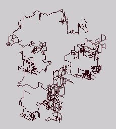
So for phenomenon that appear to depart from conventional normal diffusion (the so-called anomalous diffusion) we have two distinct camps and corresponding solution paths to choose from. The prevailing wisdom suggests that an entirely different kind of random walk occurs (Camp 1). No longer does the normal diffusion apply, giving rise to normal statistics; instead we get the statistics of fat-tails and random walk trajectories called Levy flights to concretely describe the situation (see Figure 1). The mathematics quickly gets complicated here and most of the results get cast into heuristic power-laws. It takes a leap of faith to follow these arguments.

The question comes down to whether we wish to ascribe anomalous diffusion as a strange kind of random walk (Camp 1) or simply suggest that heterogeneity in diffusional and drift properties adequately describes the situation (Camp 2). I take the stand in the latter category and stand pretty much alone in this regard. Find some academic research article on anything related to anomalous diffusion and very few will accept the most parsimonious explanation -- that a range of diffusion constants and mobilities explain the results. Instead the researcher will punt and declare that some abstract Levy flight describes the motion. Above all I would rather think in practical terms, and simple variability has a very pragmatic appeal to it.

I went through the derivation of the dispersive FPE solution for a disordered semiconductor in the last post, and want to generalize it here. This makes it especially applicable to notions of transport physical transport of material in porous matter. This would include the motion of oil underground, CO2 in the air, and perhaps even spilled oil at sea.

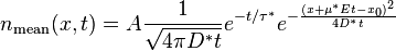
In the one-dimensional model of applying an impulse function of material, the concentration n will disperse according to the following equation:
n(x, z) = (z + sqrt(zL + z^2)/sqrt(zL + z^2)*exp(-2x/(z + sqrt(zL + z^2))

where
z= μFt
L = β/F
The term z takes the place of a time-scaled distance, which can speed up or slow down under the influence of a force F (i.e. gravity, or electric field for a charged particle). The characteristic distance L represents the effect of the stochastic force β (aka Boltzmann's constant) and ties in the diffusional aspects of the system. The specific parameterization of the exponential results in the fat-tail observed.

In the past, I had never gone through the trouble of solving the FPE, simply because intuition would suggest that the dispersive envelope would cancel out most of the details of the diffusion term. In the dispersive transport model that I originally conceived, the dispersion would at most follow the leading wavefront of the drifting diffusional field as "sqrt(Lz+z^2)" as described here or as "sqrt(Lz)+z" here.

I estimated that the diffusion term would follow as the square root of time according to Fick's first law and that drift would follow time linearly, with only an idea of the qualitative superposition of the terms in my mind.

As one might expect, the actual entropic FPE solution borrowed from a little of each of my estimates, essentially averaging between the two:
(z + sqrt(zL + z^2))/2
So the solution to the dispersive FPE form for a disordered system turns out entirely intuitive , and one can almost generate the result from inspection. The difference between the original entropic dispersion derivation and the full FPE treatment amounts to a bit of pre-factor bookkeeping in the first equation above. You can see this by comparing the two approaches for the case of L=1 and unity width for the dispersive transport current model.

Figure 2: Differences between the original entropic dispersive model and the fully quantified FPE solution will converge as L gets smaller.

Dispersive Transport in Porous Media.

The above solved equations can actually apply directly as solutions to Darcy's law when it comes to describing the flow of material in a disordered porous media. I suppose this will irk the petroleum engineers, hydrologists, and geologists out there who have long sought the solution to this particular problem.

Yet we should not act surprised by this result. The actions of multiple processes acting concurrently on a mobile material will generally result in a universal form governed by maximum entropy. It doesn't matter if we model carriers in a semiconductor or particles in a medium, the result will largely look the same. In a hydraulic conductivity experiment, Lange treated the breakthrough curve of a trace element through a natural catchment as a FPE convection-dispersion model, and came up with the same results independent of the fractionation of the media.

By applying the simple dispersion model (blue curve below) to Lange's results, one sees that an excellent fit results with the fat-tail exactly following the hyperbolic decline that reservoir engineers often see in long-term flow behavior. This could includes the time dependent emptying of the currently leaking deep sea Gulf reservoir!

Figure 3: Breakthrough curve of a traced material showing results from an entropic dispersion model in blue.

Moreover, the amount of diffusion that occurs appears quite minimal. Adding a greater proportion of diffusion by increasing L does not improve the fit of the curve (see the chart to the right). Just as in the semiconductor case, the shape has a significant meaning when analyzed from the perspective of maximum entropy.

Nothing complicated about this other than admitting to the fact that heterogeneous disordered systems appear everywhere and we have to use the right models to characterize their behavior.

The details of this experiment are described in the following papers:
  1. D.Haag and M.Kaupenjohann, Biogeochemical Models in the Environmental Sciences: The Dynamical System Paradigm and the Role of Simulation Modeling
  2. H. Lange, Are Ecosystems Dynamical Systems?
The authors of these papers have mixed feelings about the applicability of modeling biogeochemical systems and speculate whether we should use any kinds of models for "ecological risk assessment". They point out that ecological systems obviously can adapt under certain circumstances and no amount of physical modeling can predict which way the system will go. Will spilled oil decompose faster as the environment adapts around it? Will that make dispersion less relevant? Who knows?

Still the work of modeling the physical process alone has enormous value as Haag and Kaupenjohann point out:

Despite not being a ‘real’ thing, "a model may resonate with nature" (Oreskes et al. 1994) and thus has heuristic value, particular to guide further study. Corresponding to the heuristic function, Joergensen (1995) claims that models can be employed to reveal ecosystem properties and to examine different ecological theories. Models can be asked scientific questions about properties. According to Joergensen (1994), examples for ecosystem properties found by the use of models as synthesizing tools are the significance of indirect effects, the existence of a hierarchy, and the ‘soft’ character of ecosystems. However, we agree with Oreskes et al. (1994) who regard models as "most useful when they are used to challenge existing formulations rather than to validate or verify them". Models, as ‘sets of hypotheses’, may reveal deficiencies in hypotheses and the way biogeochemical systems are observed. Moreover, models frequently identify lacunae in observations and places where data are missing (Yaalon 1994).

As an instrument of synthesis (Rastetter 1996), models are invaluable. They are a good way to summarize an individual research project (Yaalon 1994) and they are capable of holding together multidisciplinary knowledge and perspectives on complex systems (Patten 1994).

While models as a product may have heuristic value, we would like to emphasize also the role of the modeling process: "[…] one of the most valuable benefits of modeling is the process itself. These benefits accrue only to participants and seem unrelated to the character of the model produced" (Patten 1994). Model building is a subjective procedure, in which every step requires judgment and decisions, making model development ‘half science, half art’ and a matter of experience (Hoffmann 1997, Hornung 1996). Thus modeling is a learning process in which modelers are forced to make explicit their notions about the modeled system and in which they learn how the analytically isolated components of a system can be ‘glued’ (Paton 1997). As modeling mostly takes place in groups, modeling and the synthesis of knowledge has to be envisaged as a dynamic communication process, in which criteria of relevance, the meaning of terms, the underlying concepts and theories, and so forth are negotiated. Model making may thus become a catalyst of interdisciplinary communication.

In the assessment of environmental risks, however, an exclusively scientific modeling process is not sufficient, as technical-scientific approaches to ‘post-normal’ risks are unsatisfactory (Rosa 1998) and as the predictive capacity and operational validity of models (e.g. for scenario computation) is in doubt. The post-normal science approach (Funtowicz & Ravetz 1991, 1992, 1993) takes account of the stakes and values involved in environmental decision making. Following a ‘post-normal’ agenda, model development and model validation for risk assessment should become a trans-scientific (communication) task, in which "extended peer communities" participate and in which non-equivalent descriptions of complex systems are made explicit, negotiated, and synthesized. In current modeling practice, however, models are highly opaque and can rarely be penetrated even by other scientists (Oreskes, personal communication). As objects of communication, models still are closed systems and black boxes.

We need to really take up the charge on this as our future depends on understanding the role of entropy in nature. For too long, we have not shown the intellectual curiosity to model how much oil we have underground, what size distribution the reservoirs take, and how fast that they can epmty, even though some perfectly acceptable models can describe this statistically, using dispersion no less!

Now that the Macondo oil has discovered an escape hatch and has gone disordered on us and will go who-knows-where, it seems we can really make some headway in our common understanding. Nothing like having your feet in the fire.

Real GDP increases 2.9%


Real GDP rose 2.9% in the third quarter of 2007 (Chart 1). Domestic demand growth remained solid, with real final domestic demand and inventory investment both contributing to the gain. The increase in real final domestic demand outpaced that of real GDP for the 11th time in the last 12 quarters as real imports rose more than real exports.

Consumer spending stays healthy

Real consumer expenditure grew 3.0% in the third quarter of 2007, following a gain of 5.9% in the previous quarter. Spending on semi-durable goods and services (notably net spending abroad) increased, while that on durable goods (especially automotive products) and non-durable goods fell.

Chart 1 - Growth in real GDP and real final domestic demand

Gains in income growth have supported household spending. Personal income increased 1.1% in the quarter. Supported by higher employment, labour income rose 1.9%, albeit a slowdown from 7.2% in the second quarter. This slowing reflected the end of Quebec government pay equity payments and special contributions from the Newfoundland and Labrador government to its Public Service Pension Plan. These factors had boosted labour income in the first half of 2007.

In the third quarter, real personal disposable income rose 2.4% and per capita real personal disposable income increased 1.1%. The personal savings rate was 1.3%, down from 1.6% in the second quarter.

Oil Prices: A Year After a Record $145, Gloom Prevails

Friday is the one-year anniversary of crude oil’s record close of $145 a barrel. But commodity traders were in no mood for a party.

dismayed_oil_trader_DV_20090702122041.jpg

Oil prices dropped more than $2 a barrel to below $67 in trading in New York Thursday, beaten down by dismal economic news and word that the Organization of Petroleum Exporting Countries discipline is shaky.

First news out of the U.S., the world’s largest consumer of crude oil: the unemployment rate is up to 9.5%, the highest since Ronald Reagan’s first term in office; and the federal government reported payrolls tumbled. Our Dow Jones Newswires colleague noted there were “widespread declines across manufacturing, construction and professional services, a grim reminder that the path to economic recovery will be bumpy.” (Sub. req’d.) The jobless rate in the Eurozone is also at 9.5%, a 10-year high. More unemployment means more insecurity, less spending and less fossil-fuel consumption.

But this might not even be the worst news for oil bulls. Months of big OPEC production cuts have been a primary factor for the sweeping recovery in crude prices. But that hardnosed disciplined is wavering as a steady stream of increased production from some of the cartel’s members quietly enters the market.

A Dow Jones Newswires’ survey Thursday shows output from OPEC’s 11 quota-bound members rose a third straight month in June. Led by Iran and Venezuela, output was up almost 300,000 barrels a day, or 1%, compared with March.

OPEC compliance with a trio of large output reductions announced late last year is now at 76%, down seven percentage points, since March, according to the survey. Some other industry reports though have OPEC compliance near just 70%.

“Creeping OPEC production serves to underscore the underlying weakness (of the market) and that (prices) likely got ahead of themselves,” says PFC Energy analyst David Kirsch.

Moody’s, the credit rating agency, says Thursday its forecast for the global integrated oil industry is “negative” as it expects economic recovery in 2010 to be “slow and painful, crimping worldwide demand for oil and natural gas at a time when inventories are near record highs.”

Of course, it bears repeating that weakness in crude-oil markets doesn’t mean strength for renewable sources of energy. Biofuels as well as wind and solar still need energy prices to be high to help them claw their way to profitability. A collapse in oil prices will be bad news for boosters of carbon-lite fuel.

Monday, May 24, 2010

Fokker-Planck for Disordered Systems

To get the cost of photovoltaic (PV) systems down, we will have to learn how to efficiently use crappy materials. By crap I mean that mass-produced PV materials will end up getting rolled or extruded or organically grown. Unless we perfect the process, most everything will turn out non-optimal. We already know the difference between clean-room cultivated single crystal semiconducting material and the defect-ridden and often amorphous materials that nature and entropy drives us to. For performance sensitive applications such as communications and computing we would only rarely consider disordered material as a candidate semiconductor. Certainly, the performance of these materials makes them unlikely candidates for high speed processing -- yet for solar cell applications, they may serve us well. In the end, we just have to learn how to understand and deal with crap.

The following will revisit a couple of previous posts where I outlined a novel way to analyze the behavior of disordered semiconducting material. I know for certain that no one has proposed the particular approach before. If it does exist, I certainly can't find it in the literature. From one perspective, this analysis sets forth a baseline for the characterization of a maximally disordered semiconductor.

Background

The prehistoric 1949 Haynes-Shockley experiment first measured the dynamic behavior of charged carriers in a semiconducting sample. It basically confirmed the solution of the diffusion (Fokker-Planck) equation and it demonstrated diffusion, drift, and recombination in a conceptually simple setup. This animated site gives a very interesting overview of PV electrical behavior.

Figure 1: Apparatus for the Haynes-Shockley experiment

This setup works according to theory for an ordered semiconductor with uniform properties but apparently gets a bit unwieldy for any disordered or non-uniform material sample. I inferred this as conventional wisdom since most scientists either punt or use heuristics partially derived from the inscrutable work of a select group of random-walk theorists (see Scher & Montroll).

I had previously applied a very straightforward interpretation to the problem of carrier transport in disordered material. My dispersion analysis essentially set aside the Fokker-Planck formalism for a mean value approximation where I tactically applied the Maximum Entropy Principle. In particular, I really like the MaxEnt solution because I can recite the solution from memory. It matches intuition in a conceptually simple way once you get into a disordered mind-set.

In the real Haynes-Shockley experiment, a pulse gets injected at one electrode, and a nearly pure time-of-flight (TOF) profile results. The initial pulse ends up spreading out in width a bit, but the detected pulse usually maintains the essential Gaussian sigmoid shape.

Adding Disorder

For the time-of-flight for a disordered system, the Maximum Entropy solution looks like:
q(t) = Q * exp(-w/(sqrt((μEt)2 + 2Dt))
This essentially states that the expected amount of charge accumulated at one end of the sample (at a distance w) at time t, follows a maximum entropy probability distribution. The varying rates described by μ and D disperse the speed of the carriers so that a broadened profile results from the initial pulse spike.

The equation above formed the baseline for the interpretation I described initially here.

For completeness, I figured to test my luck and see if I can bull my way through the basic diffusion laws. If I could produce an equivalent solution by applying the Maximum Entropy Principle directly to the Fokker-Planck equation, then this would give a better foundation for the "inspection" result above.

The F-P diffusion equation gets expressed as a partial differential equation with a conservation law constraint:
In this case D1=μ* (carrier mobility) and D2=D* (diffusion coefficient), and f(x,t)=n(x,t) (carrier concentration). With recombination, the solution in one-dimension looks like:

This of course works for well-ordered semiconductors, but D* and μ* will likely vary for disordered material. I made the standard substitution via the Einstein Relation for
D* = Vt μ*
where Vt = β/q stands for the chemical or thermal potential at equilibrium (usually β equals kT where k is Boltzmann's constant and T is absolute temperature). At equilibrium, the stochastic force of diffusion exactly balances the electrostatic force F = qE.

From the basic physics, we can generate a maximum entropy density function for D
p(D*) = 1/D * exp(-D*/D)
then
n(x,t) = Integral p(D*) * nmean(x,t) over all D*
This looks hairy but the integral comes out straightforwardly as (ignoring the constant factors)
n(x,t) = 1/sqrt(t*(4D+t*(Eμ)2)) * exp(-x*R(t)) / R(t)
where
R(t) = sqrt(1/(Dt) + E/(2Vt)2) - E/(2Vt)

If we evaluate this for carriers that have reached the drain electrode at x=w, the total charge collected q is:
q(t) = Q/sqrt(t*(4D+t*(Eμ)2) * exp(-w*R(t)) / R(t)

The measured current is
I(t) = mean of dq(t)/dt from 0 to w
The simple entropic dispersive expression and the Fokker-Planck result obviously differ in their formulation, yet the two show the same asymptotic trends. For an arbitrary set of parameters, one can't detect a practical difference. Use whichever you feel comfortable with.

I show the dynamics of the carrier profile in the animated GIF to the right. The initial profile starts with a spike at the origin and then the profile broadens as the mean starts drifting and diffusing to the opposing contact. You don't see much from this perspective as it looks completely like mush. Yet, when plotted on a log-log scale, it does take on more character.

The collected current profile looks like the following

Figure 2: Typical photocurrent trace showing the initial diffusional spike, a plateau for relatively constant collection from the active region, and then a power-law tail produced from the entropic drift dispersion.


Organic Semiconductor Applications

The photocurrent profile displayed above came from from Andersson's "Electronic Transport in Polymeric Solar Cells and Transistors" (2007) wherein he analyzed the transport in a specific organic semiconducting material, the polymer APFO.

The blue line drawn through the set of traces follows the entropic dispersion formulation. The upper part of the curve describes the diffusive spike while the lower part generates the fat-tail due to the drift component (this shows an inverse square power law in the tail).

Figure 3: Universal profile generated over a set of applied electric field values. For this set, scaling of transit time with respect to the applied field holds, indicative of a constant mobility. However, carrier diffusion causes the initial transient and this does not scale, as the electric field has no effect on diffusion, as shown in the lower set of blue curves.

As I stated in the previous post, most scientists when discussing this shape have either (1) referred to Scher/Montroll and the vague heuristic α, (2) dismissed these features, or (3) labelled them as uninteresting. Andersson follows suit:
At best this transient, as the high α value indicates, might be possible to evaluate in a meaningful way with a bit of error and at worst it is of no use. Either way the amount of material and effort required is rather large compared to the usefulness of the results. APFO-4 is also the polymer that, among the investigated, gives the ”nicest” transients. The conclusion from this is that if alternative measurement techniques can be used it is not worthwhile to do TOF.
Not to dismiss the hard work that went into Andersson's experiment, but I would beg to differ with his assessment of the worthiness of the approach. When characterizing a novel material, every measurement adds to the body of knowledge, and as the interpretation of the aggregation of data becomes more cohesive, we end up learning much more of the internal structure. As I have learned, if someone does not understand a phenomena, they tend to dismiss it (myself included).

By their very nature, disordered systems contain a huge state space and we really can't afford to throw out any information.

Which brings up another interesting set of TOF experiments that I dug up. These also deal with organic semiconducting materials -- the polymers with the abbreviations ANTH-OXA6t-OC12 and TPA-Cz3d. The following figures show the TOF results for various applied voltages. I superimposed the entropic dispersion equation form as the red line with the derived mobility in the caption below each figure. The original researcher had applied the Scher&Montroll Continuous Time Random Walk (CTRW) heuristic as indicated by the intersecting sloped lines. The CTRW model clearly fails in this situation as the slopes need quite a bit of creative interpretation. Note that we don't observe the diffusive spike; I integrated the charge from 10% to 100% of the width instead of 0% to 100%.


ANTH-OXA6t-OC12
μ = 0.0025
TPA-Cz3d
μ = 0.0013
μ = 0.00155
μ = 0.0004
μ = 0.00125
μ = 0.0005
μ = 0.00085
μ = 0.0006


The number of papers I find, especially when dealing with organic semiconductors, that cannot apply the Scher/Montroll theory indicates that it truly lacks any generality. In other words, it works crappily for describing disorderly crap. I will also say the theory has some very serious flaws, including the claim that an α = 1 defines a non-dispersive material. How could a power-law of -2 be anything but dispersive?

The fact that the entropic dispersion formulation works on any disordered material makes it much more general. Several years ago Scher wrote a popular article for Physics Today extolling the wonders of his theory, and how it seemed to fit a variety of disordered systems. He mentioned how well it fit amorphous silicon based on the number of orders of magnitude that his piece-wise line segments matched. Well, the entropic dispersion does just as well:

And nothing mysterious about that slope of 0.5; that results from the diffusion having a square root dependence with time.

Friday, May 21, 2010

Waste Half-Life

The big Gulf Spill got me thinking about the half-life of the leaking crude oil and the expanding slick. First of all, the oil will biodegrade over time. We don't have the situation as in CO2 where a sizable fraction will wander around the atmosphere trying to find a suitable location to react and form solutes.

Most of the oil will stay on the surface where it will get plenty of attention from aerobic microoganisms. Some of the oil will sink into the ocean and find anaerobic conditions at the bottom and essentially become inert or wash up on shore as sticky globs. Also the composition of crude oil includes many different hydrocarbons, some of which biodegrade at much slower rates, due to their molecular structure.

So I imagine that we can't calculate the half-life of the spilled oil in terms of a single rate constant, k. This kind of first-order kinetics would likely show an exponential decline, which proceeds pretty quickly once you get past the half-lifetime, 1/k . Instead we will get a mix of various rates, with the fast rates occurring initially and the slower rates picking up the slack.

Radioactive waste-dumps also show a mix of decay constants. Nominally, radioactive material will show a single Poisson emission rate, leading to an exponential decline over time. But when the different radioactive materials get combined, the Geiger counter will pick up this mixture of rates, and the decline will turn from an exponential to a fat tail distribution See the red curve below.


A maximum entropy mix of decay rates (where a high decay rate indicates a potentially more energetic state) will generate the following half-life decline profile:
P(t) = 1/(1+k*t)
where k is the average of the individual rates. This looks exactly the same as the hyperbolic decline of reservoirs in my last post.

As you can see, the combined activity shows a much larger equivalent half-life since the tail has so much meat in it. In the limit of a full dispersion of rate constants, the average half-life will actually slowly diverge as the log of infinity. However, it never reaches this because the slowest decay rate will eventually dominate and that will not diverge.

In any case, this gives a good qualitative description of a random waste dump.

If I make the same MaxEnt assumption for crude oil and assume that the most energetic oil (by the bond strength of the hydrocarbon [1]) will likely prove the most difficult to decompose, then the half-life may also show a similar kind of fat-tail as that of a waste dump. It looks like benzene breaks down much slower than diesel oil for example.

As usual, disordered natural phenomena show many of the same dispersive characteristics, driven largely by maximizing entropy.


Notes:

[1] For the derivation, we assume that we have a mean energy E0 and then a probability density function will show many small energies and progressively fewer high energies.
p(E) = exp(-E/Eo)/E0
but the decomposition rate R depends on E, so that
P(t) = integral of P(t|E)p(E) over all E
P(t|E) = exp(-kE*t)

P(t) = 1/(1+tkEo)

(See this for a more detailed derivation.)

Tuesday, May 18, 2010

Hyperbolic Decline a Fat-Tail Effect

If the Gulf Oil spill shows results of a hyperbolic decline, the effects can go on for quite some time.

For a typical reservoir, oil depletion goes through either an exponential decline or a hyperbolic decline. Geologists by and large don't realize this, and definitely don't teach this, but hyperbolic decline constitutes a "fat-tail" effect that results from an aggregation of varying exponential declines summed together. As to the behavior of hyperbolic decline, one notices that the effects tend to drag out for a long time. The fast exponential decline finishes more quickly than the slower exponential components. That's where the fat-tail comes from and why the hyperbolic decline can proceed endlessly are at least as long as the longest exponential portion.

Derivation of hyperbolic decline as a one-liner:

The exponential has a rate of x, and x gets integrated over all possible values of r according to an exponential Maximum Entropy probability density function. You can see the fat-tail in the plot below:


This is just entropy at work because nature tends to want to disperse.

EDIT:

JB asked the question on the slope of the two functions. As plotted, these give the cumulatives. If we want to look at the probability density functions, then yes you will see that the hyperbolic gives a mix of these rates more in line with intuition, with a faster initial slope and then the fatter tail later. See the figure below:


petroleum


Petroleum was formed from the remains of marine plant and animal life which existed many millions of years ago (hence it is known as a fossil fuel). Some of these remains were deposited along with rock-forming sediments under the sea where they were decomposed anaerobically (without oxygen) by bacteria which changed the fats in the sediments into fatty acids which were then changed into an asphaltic material called kerogen. This was then converted over millions of years into petroleum by the combined action of heat and pressure. At an early stage the organic material was squeezed out of its original sedimentary mud into adjacent sandstones. Small globules of oil collected together in the pores of the rock and eventually migrated upwards through layers of porous rock by the action of the oil's own surface tension (capillary action), by the force of water movement within the rock, and by gas pressure. This migration ended either when the petroleum emerged through a fissure as a seepage of gas or oil onto the Earth's surface, or when it was trapped in porous reservoir rocks, such as sandstone or limestone, in anticlines and other traps below impervious rock layers.

The modern oil industry originates in the discovery of oil in western Ontario in 1857 followed by Edwin Drake's discovery in Pennsylvania in 1859. Drake used a steam engine to drive a punching tool to 21 m/68 ft below the surface where he struck oil and started an oil boom. Rapid development followed in other parts of the USA, Canada, Mexico, and then Venezuela where commercial production began in 1878. Oil was found in Romania in 1860, Iran in 1908, Iraq in 1923, Bahrain in 1932, and Saudi Arabia and Kuwait in 1938.

The USA led in production until the 1960s, when the Middle East outproduced other areas, their immense reserves leading to a worldwide dependence on cheap oil for transport and industry. In 1961 the Organization of the Petroleum Exporting Countries (OPEC) was established to avoid exploitation of member countries; after OPEC's price rises in 1973, the International Energy Agency (IEA) was established in 1974 to protect the interests of oil-consuming countries. New technologies were introduced to pump oil from offshore and from the Arctic (the Alaska pipeline) in an effort to avoid a monopoly by OPEC. Global consumption of petroleum in 1993 was 23 billion barrels.

As shallow-water oil reserves dwindle, multinational companies have been developing deep-water oilfields at the edge of the continental shelf in the Gulf of Mexico. Shell has developed Mars, a 500-million-barrel oilfield, in 900 m/2,940 ft of water, and the oil companies now have the technology to drill wells of up to 3,075 m/10,000 ft under the sea. It is estimated that the deep waters of Mexico could yield 8–15 million barrels in total; it could overtake the North Sea in importance as an oil source.


Petrol prices hit record high and could increase even more


Petrol prices look set reach £6 per gallon, and rising. Photograph: Graham Turner

The following correction was printed in the Guardian's Corrections and clarifications column, Tuesday 13 April 2010

petrol prices

This sentence read as though it was expressing national totals: "Supermarkets operate just 1,200 of the 10,000 petrol stations in the UK, but they account for an average of 12m litres of the 14.5m litres of petrol sold each year." What the writer meant was that each of the 1,200 supermarket sites sold an annual average of 12m litres, and the others each sold 2.5m litres a year


Petrol prices reach £5 a gallon


The average motorist could soon be paying more than £2,600 a year to fill up their car, swallowing almost 15 per cent of the average take-home pay, a survey predicted.

Figures compiled by the AA showed that on Tuesday the national average price for a litre of unleaded petrol rose to 110.2p, or £5.01 a gallon. Diesel now costs 120.51p, or £5.48 a gallon.

Edmund King, the president of the AA, described the record high as "the latest milestone along a miserable road of increasing fuel prices this year".

Soaring costs of crude oil, caused by increased demand from developing countries such as China and India, have pushed up petrol prices by almost 20p a litre since this time last year.

Meanwhile, oil companies have been accused of ripping off motorists after BP and Shell announced record profits totalling more than £7 billion for the first three months of this year.

But a comprehensive study by uSwitch.com, the comparison website, suggests much worse is to come. Many analysts have suggested that by next year petrol could cost 150p per litre, meaning the average car would cost £84 to fill, compared with £49.22 last year.

For a motorist driving 12,000 miles a year, that equates to £2,636 in annual fuel bills – £706 more than this year.

Even smaller cars, such as Ford Fiestas, would cost £1,792 a year to fill up, while a luxury saloon such as a Mercedes C-Class would cost £4,190.

The average net salary in 2009 is predicted to be £19,167, meaning the average car will guzzle 14 per cent of take-home pay in fuel bills alone.

Ann Robinson, of uSwitch.com, said: "Unfortunately the outlook for drivers is bleak. This latest blow could be enough to force some drivers off the road altogether. As a direct result of these price hikes, it would be no surprise to see more motorists leaving their car at home and using other methods of transport.

"However, drivers who are reliant on their cars for business or live in remote areas will be hardest hit - for them, leaving the car at home is not an option."

Gordon Brown is under increasing pressure to scrap a 2p increase in fuel duty planned for October or even to cut fuel duty after hauliers warned that hundreds of companies would go out of business if the price rises continued.

Petrol Prices


Since March 1983 I have kept a detailed record of fuel prices and fuel consumption, spanning fourteen different cars, both privately-owned and company. This table records the movement in fuel prices over that period, taking in each year the first fuel purchase in March. Prices are for leaded 4-star up to 1988, and unleaded thereafter. This roughly corresponds to the point when unleaded took over from 4-star as the standard fuel.

The table shows that the price of fuel in real terms is now 15% higher in March 2010 than in 1983, the oil price having risen steadily since March 2009, and the price also having been affected by the weakness of the pound against the dollar. The real terms price is now a record for the period covered, and is over 50% higher than in 1990. During the period covered by the table, "real" fuel prices fell between 1983 and 1992, encouraging a boom in road traffic, but then rose sharply due to the "fuel duty escalator", resulting in the fuel protest of 2000. At this time, fuel prices had risen by over 50% in five years, which undoubtedly caused much hardship.

Petrol Prices 1983-2010
Year Price per Litre (p) Price per Gallon (£) Retail
Prices
Index
Petrol Price
in constant terms
(1983=100)
5-year
% increase 
1983 36.7 1.670 83.1 100.0 -
1984 38.7 1.759 87.5 100.0 -
1985 42.8 1.946 92.8 104.3 -
1986 38.2 1.737 96.7 89.4 -
1987 37.8 1.719 100.6 85.0 -
1988 34.7 1.578 104.1 75.4 -5.5
1989 38.4 1.746 112.3 77.4 -0.7
1990 40.2 1.828 121.4 74.9 -6.1
1991 39.5 1.796 131.4 68.0 3.4
1992 40.3 1.832 136.7 66.7 6.6
1993 45.9 2.087 139.3 74.6 32.3
1994 48.9 2.223 133.1 77.6 27.3
1995 50.9 2.314 147.5 78.1 26.6
1996 52.9 2.405 151.5 79.0 33.9
1997 57.9 2.632 155.4 84.3 43.7
1998 60.9 2.769 160.8 85.7 32.7
1999 61.9 2.814 164.1 85.3 26.6
2000 76.9 3.496 168.4 103.3 51.1
2001 77.9 3.541 173.1 101.8 47.2
2002 69.9 3.178 174.5 90.6 20.7
2003 77.9 3.541 179.9 98.0 27.9
2004 77.9 3.541 184.6 95.5 25.8
2005 79.9 3.632 190.5 95.0 3.9
2006 88.9 4.041 195.0 103.2 14.1
2007 87.9 3.996 204.4 97.4 25.6
2008 103.9 4.723 212.1 110.9 33.4
2009 89.9 4.087 211.3 96.2 15.4
2010 111.9 5.087 220.7 114.8 40.1

The table also does not show peak prices in my local area, which were 224.6p/gallon (49.4p/litre) in October 1990, following the Iraqi invasion of Kuwait, and 390.5p/gallon (85.9p/litre) in June 2000, just before the fuel protest. Around this time I even paid 404.1p/gallon (88.9p/litre) in the Scottish Highlands. It seems that peak prices tend to occur in the autumn, and March, just as winter demand is tailing off, is often a low point in the year.

In 2005 there was a marked rise in the international price of oil, leading to a peak price of 426.9p/gallon (93.9p/litre) in September and October. Also since the beginning of March 2008 there was a further sharp spike in the international oil price, with unleaded reaching a startling peak in July of 540.5p/gallon (118.9p/litre). Recently, the price has continued to increase after the beginning of March, with my most recent fill-up having been at a personal record of 545.1p/gallon (119.9p/litre).